本篇主要学习一下符号同步相关的技术, 特别是timing 同步的环路, 这里的环路指的并不是PLL。
Timing 环路的构成
时间同步环路常由TED, 环路滤波器, VCO构成, 如下下图所示[1]:
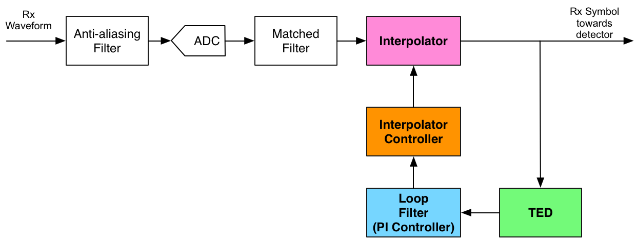
对于离散时间系统来说, 第n个接收到的符号可以用下面的模型来表示:
$T_s$是符号的周期, p 是信道的冲激响应, 对于上图中的模型来说, 包含了发端的pulse shape filter 和收端的match filter。
x(m) 代表的是第m个发送的符号, $v(nT_s)$这一项表示AWGN 噪声。
$\tau$ 代表的是范围在[0, $T_s$)内的timing 误差。 实际上由于信道的传输延时造成的timing error 可能由两部分构成:
a. 整数倍的$T_s$;
b. 小数倍的$T_s$;
对于timing loop来说, 我们关心的是小数倍的timing error, 而整数倍的timing error 可以由帧同步来修正。
TED
TED 的作用就是检测上文中提到的timing error $\tau$, 值得注意的是, 由于$\tau$ 的存在会有符号间的干扰, 常见的接收机结构是需要进行符号级的均衡后再进行判决。
Loop Filter
Loop Filter的基本概念就是能够决定修正timing error的快慢, 什么类型的timing error 可以被修正, 以及多大范围的时间误差可以被修正。
通常来说这部分是一个二阶系统, 可以看做是一个比例积分控制器(PI controller)
Interpolator
插值控制器对于timing loop 来说是很重要的一个组件。 比如, 过采样因子为L=4, 那么每一个symbol 的输出就会有L 个sample。那么接收机必须选择这4个sample 中的一个进行符号检测或者判决。
下面我们以PAM符号收发系统为例子, 用MATLAB详细说明timing 同步环路的作用
PAM 系统中的timing 同步
分三部分, 以MATLAB 代码和图片进行说明。
PAM的发送
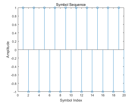
如下所示:PAM 2 {+1, -1 ,+1, -1 …}符号产生
1 | L = 4; % Oversampling factor |
PAM 2符号为:
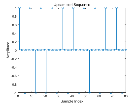
PAM2 4倍上采样后的sample为:
1 | % Upsampling |
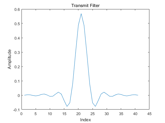
pulse shape
pulse shape 滤波器在发端symbol 产生之后, 用于频谱整形, 使之在通信标准的模板(Mask)之内. 以根升余弦滤波器为例:
1 | L = 4; % Oversampling factor |
发端滤波器响应为:
收端match filter 的响应为:
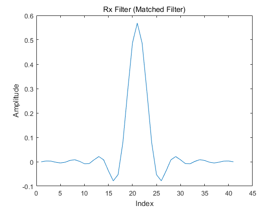
收发端滤波器的整体响应和过零点:
Channel
为了便于说明, 我们先忽略channel中的AWGN, 并且增加一定的延时(比如一个采样间隔), 注意这里的采样间隔并不等同于符号间隔:
1 | timeOffset = 1; % Delay (in samples) added |
Receiver
- 没有符号同步的情况:
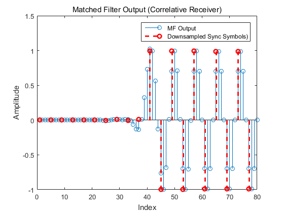
我们先假设接收机中没有符号的定时同步,那么经过match filter收端收到的符号就是:
1 | mfOutput = filter(hrx, 1, rxDelayed); % Matched filter output |
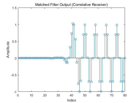
针对MF 输出, 任意选择sample送给符号判决器:
1 | rxSym = downsample(mfOutput, L); |
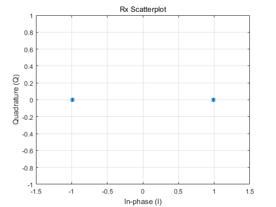
最后, 画出接收符号的散点图:
1 | figure |
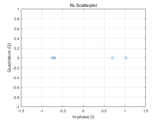
可以看出接收的符号已经偏离了+1 和 -1
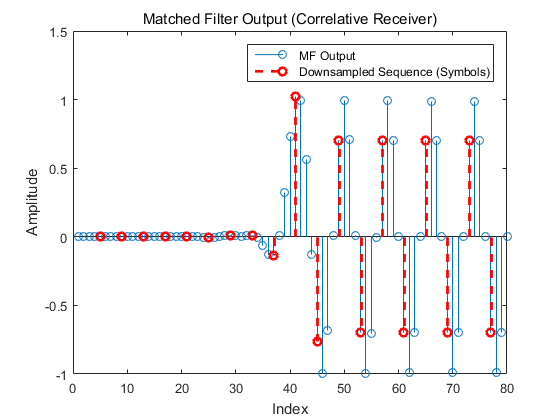
- 有符号同步的情况
在downsample 函数中增加一个TimeOffset的值:
1 | rxSym = downsample(mfOutput, L, timeOffset); |
这种情况下, 被选择的符号就是:
1 | selectedSamples = upsample(rxSym, L); |
画出散点图:
TED 设计
本部分我们讨论Timing Error的检测.。
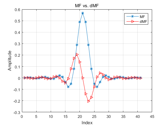
TED 中的一种是最大似然检测, 即(ML-TED), 这种检测器使用的是微分式的匹配滤波器:
1 | h = [0.5 0 -0.5]; % central-differences kernel function |
可以看到dMF响应的零点对应MF 响应的peak点。
ML-TED
那么经过dMF后, 下采样的sample为:
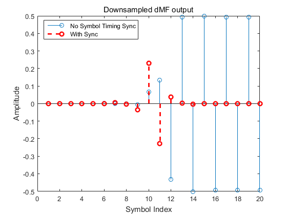
计算timing error:
1 | % First do PAM-demodulation |
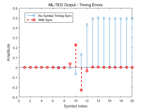
从图中可以看出, 当receiver 不知道TimeOffset的信息时, TED的输出有较大的幅值, 因此可以利用这个误差值来获取同步。
但是需要注意的是, ML-TED要求发端发送固定的pattern, +1 , -1, +1, -1等。 当发送的是随机的symbol时候, ML-TED的输出就会有很多噪声, 影响timing loop稳定性。
ZC-TED(Zero-Crossing)
Zero-crossing 方法的timing error检测不需要dMF, 只需要MF输出的sample。因为每两个symbol 之间有L-1的sample, 当MF的输出存在极性转换时(+1 —> -1),就可以用中间这个sample的值作为TED的输出:
以下图为例, MF的输出从+1 到 -1 转换时, 可以取 Index = 3的sample作为TED的输出:
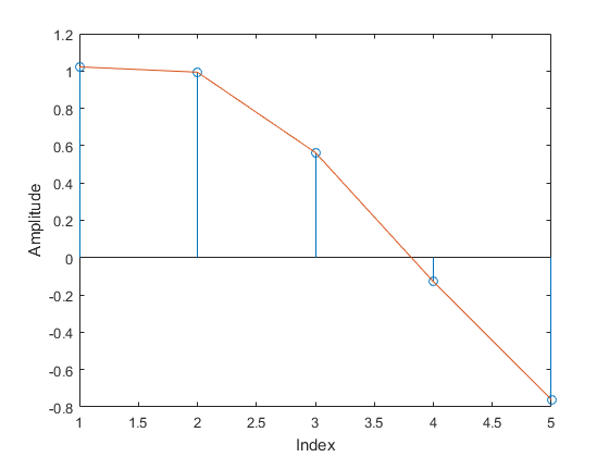
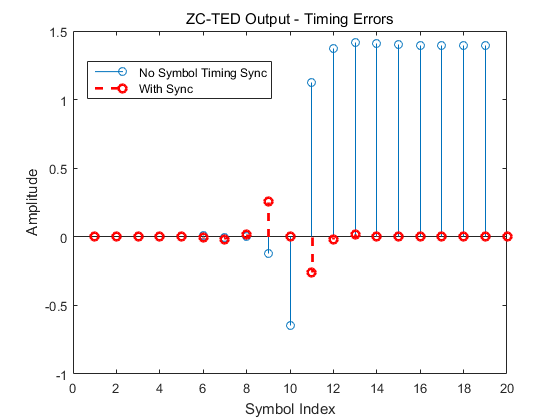
那么据此, 可以得到ZC-TED的输出:
1 | % Midpoint samples |
如下图所示:
参考文献
[1] http://igorfreire.com.br/symbol-timing-synchronization-tutorial/#wireless-communications-fpga-course
[2] Rice, Michael. Digital Communications: A Discrete-Time Approach. Upper Saddle River, NJ: Prentice Hall, 2009